How to simulate multiple virus strains
In this tutorial, we are going to simulate the spread of Covid-19 with two virus strains.
[19]:
%matplotlib inline

import warnings

import matplotlib.pyplot as plt
import numpy as np
import pandas as pd

import sid
from sid.config import INDEX_NAMES

warnings.filterwarnings("ignore")
Preparation
For the simulation we need to prepare several objects which are identical to the ones from the general tutorial on the simulation.
[2]:
available_ages = [
    "0-9",
    "10-19",
    "20-29",
    "30-39",
    "40-49",
    "50-59",
    "60-69",
    "70-79",
    "80-100",
]

ages = np.random.choice(available_ages, size=10_000)
regions = np.random.choice(["North", "South"], size=10_000)

initial_states = pd.DataFrame({"age_group": ages, "region": regions}).astype("category")
initial_states.head(5)
[2]:
| age_group | region | |
|---|---|---|
| 0 | 80-100 | North |
| 1 | 10-19 | North |
| 2 | 0-9 | North |
| 3 | 0-9 | North |
| 4 | 80-100 | South |
[3]:
def meet_distant(states, params, seed):
    possible_nr_contacts = np.arange(10)
    contacts = np.random.choice(possible_nr_contacts, size=len(states))
    return pd.Series(contacts, index=states.index)


def meet_close(states, params, seed):
    possible_nr_contacts = np.arange(5)
    contacts = np.random.choice(possible_nr_contacts, size=len(states))
    return pd.Series(contacts, index=states.index)


assort_by = ["age_group", "region"]

contact_models = {
    "distant": {"model": meet_distant, "assort_by": assort_by, "is_recurrent": False},
    "close": {"model": meet_close, "assort_by": assort_by, "is_recurrent": False},
}
[4]:
epidemiological_parameters = pd.read_csv("infection_probs.csv", index_col=INDEX_NAMES)
epidemiological_parameters
[4]:
| value | note | source | |||
|---|---|---|---|---|---|
| category | subcategory | name | |||
| infection_prob | close | close | 0.05 | NaN | NaN |
| distant | distant | 0.03 | NaN | NaN | |
| household | household | 0.20 | NaN | NaN |
[5]:
assort_probs = pd.read_csv("assort_by_params.csv", index_col=INDEX_NAMES)
assort_probs
[5]:
| value | note | source | |||
|---|---|---|---|---|---|
| category | subcategory | name | |||
| assortative_matching | close | age_group | 0.5 | NaN | NaN |
| region | 0.9 | NaN | NaN | ||
| distant | age_group | 0.5 | NaN | NaN | |
| region | 0.9 | NaN | NaN |
[6]:
disease_params = sid.load_epidemiological_parameters()
disease_params.head(6).round(2)
[6]:
| value | |||
|---|---|---|---|
| category | subcategory | name | |
| health_system | icu_limit_relative | icu_limit_relative | 50.00 |
| cd_immune_false | all | 365 | 1.00 |
| cd_infectious_true | all | 1 | 0.39 |
| 2 | 0.35 | ||
| 3 | 0.22 | ||
| 5 | 0.04 |
[7]:
params = pd.concat([disease_params, epidemiological_parameters, assort_probs])
Additional objects to simulate multiple virus strains
To implement multiple virus strains, we have to make the following extensions to the model.
Add a multiplier for the contagiousness of each virus to the parameters.
Prepare a DataFrame for the initial conditions.
[8]:
for virus, multiplier in [("base", 1), ("b117", 1.3)]:
    params.loc[("virus_strain", virus, "factor"), "value"] = multiplier
For the initial conditions, we assume a two-day burn-in period. On the first day, 50 people are infected with the base virus, on the second day one halve of 50 people has the old and the other halve the new variant.
Each column in the DataFrame is a categorical. Infected individuals have a code for the variant, all others have NaNs.
[9]:
infected_first_day = set(np.random.choice(10_000, size=50, replace=False))
first_day = pd.Series([pd.NA] * 10_000)
first_day.iloc[list(infected_first_day)] = "base"
[10]:
infected_second_day_old_variant = set(
    np.random.choice(
        list(set(range(10_000)) - infected_first_day), size=25, replace=False
    )
)
infected_second_day_new_variant = set(
    np.random.choice(
        list(set(range(10_000)) - infected_first_day - infected_second_day_old_variant),
        size=25,
        replace=False,
    )
)

second_day = pd.Series([pd.NA] * 10_000)
second_day.iloc[list(infected_second_day_old_variant)] = "base"
second_day.iloc[list(infected_second_day_new_variant)] = "b117"
[11]:
initial_infections = pd.DataFrame(
    {
        pd.Timestamp("2020-02-25"): pd.Categorical(
            first_day, categories=["base", "b117"]
        ),
        pd.Timestamp("2020-02-26"): pd.Categorical(
            second_day, categories=["base", "b117"]
        ),
    }
)
[12]:
initial_conditions = {"initial_infections": initial_infections, "initial_immunity": 50}
Run the simulation
We are going to simulate this population for 200 periods.
[13]:
simulate = sid.get_simulate_func(
    initial_states=initial_states,
    contact_models=contact_models,
    params=params,
    initial_conditions=initial_conditions,
    duration={"start": "2020-02-27", "periods": 365},
    virus_strains=["base", "b117"],
    seed=0,
)
result = simulate(params=params)
Start the simulation...
2021-02-25: 100%|████████████████████████████████████████████████████████████████████| 365/365 [00:44<00:00,  8.17it/s]
[14]:
result["time_series"].head()
[14]:
| region | newly_vaccinated | is_tested_positive_by_rapid_test | date | age_group | symptomatic | needs_icu | ever_vaccinated | n_has_infected | infectious | newly_infected | knows_immune | ever_infected | dead | immune | virus_strain | newly_deceased | new_known_case | knows_infectious | cd_infectious_false | |
|---|---|---|---|---|---|---|---|---|---|---|---|---|---|---|---|---|---|---|---|---|
| 0 | North | False | False | 2020-02-27 | 80-100 | False | False | False | 0 | False | False | False | False | False | False | NaN | False | False | False | -102 |
| 1 | North | False | False | 2020-02-27 | 10-19 | False | False | False | 0 | False | False | False | False | False | False | NaN | False | False | False | -102 |
| 2 | North | False | False | 2020-02-27 | 0-9 | False | False | False | 0 | False | False | False | False | False | False | NaN | False | False | False | -102 |
| 3 | North | False | False | 2020-02-27 | 0-9 | False | False | False | 0 | False | False | False | False | False | False | NaN | False | False | False | -102 |
| 4 | South | False | False | 2020-02-27 | 80-100 | False | False | False | 0 | False | False | False | False | False | False | NaN | False | False | False | -102 |
[15]:
result["last_states"].head()
[15]:
| index | age_group | region | ever_infected | immune | infectious | symptomatic | needs_icu | dead | pending_test | ... | cd_dead_true_draws | cd_needs_icu_true_draws | cd_received_test_result_true_draws | cd_infectious_false_draws | group_codes_close | group_codes_distant | date | period | n_contacts_close | n_contacts_distant | |
|---|---|---|---|---|---|---|---|---|---|---|---|---|---|---|---|---|---|---|---|---|---|
| 0 | 0 | 80-100 | North | False | False | False | False | False | False | False | ... | 20 | 6 | 1 | 11 | 16 | 16 | 2021-02-25 | 786 | 1 | 1 |
| 1 | 1 | 10-19 | North | True | True | False | False | False | False | False | ... | 1 | -1 | 2 | 9 | 2 | 2 | 2021-02-25 | 786 | 1 | 6 |
| 2 | 2 | 0-9 | North | True | True | False | False | False | False | False | ... | -1 | -1 | 1 | 11 | 0 | 0 | 2021-02-25 | 786 | 4 | 8 |
| 3 | 3 | 0-9 | North | False | False | False | False | False | False | False | ... | -1 | -1 | 4 | 5 | 0 | 0 | 2021-02-25 | 786 | 3 | 6 |
| 4 | 4 | 80-100 | South | True | True | False | False | False | False | False | ... | 32 | -1 | 1 | 3 | 17 | 17 | 2021-02-25 | 786 | 1 | 4 |
5 rows × 57 columns
The return of simulate is a dictionary with containing the time series data and the last states as a Dask DataFrame. This allows to load the data lazily.
The last_states can be used to resume the simulation. We will inspect the time_series data. If data data fits your working memory, do the following to convert it to a pandas DataFrame.
[16]:
df = result["time_series"].compute()
Let us take a look at various statistics of the sample.
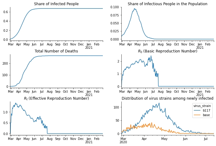
[20]:
fig, axs = plt.subplots(3, 2, figsize=(12, 8))
fig.subplots_adjust(bottom=0.15, wspace=0.2, hspace=0.4)

axs = axs.flatten()

df.resample("D", on="date")["ever_infected"].mean().plot(ax=axs[0])
df.resample("D", on="date")["infectious"].mean().plot(ax=axs[1])
df.resample("D", on="date")["dead"].sum().plot(ax=axs[2])

r_zero = sid.statistics.calculate_r_zero(df, window_length=7)
r_zero.plot(ax=axs[3])

r_effective = sid.statistics.calculate_r_effective(df, window_length=7)
r_effective.plot(ax=axs[4])

df.query("newly_infected").groupby([pd.Grouper(key="date", freq="D"), "virus_strain"])[
    "newly_infected"
].count().unstack().plot(ax=axs[5])

for ax in axs:
    ax.set_xlabel("")
    ax.spines["right"].set_visible(False)
    ax.spines["top"].set_visible(False)

axs[0].set_title("Share of Infected People")
axs[1].set_title("Share of Infectious People in the Population")
axs[2].set_title("Total Number of Deaths")
axs[3].set_title("$R_0$ (Basic Reproduction Number)")
axs[4].set_title("$R_t$ (Effective Reproduction Number)")
axs[5].set_title("Distribution of virus strains among newly infected")

plt.show()