How to resume a simulation
This tutorial shows how to resume a simulation with the states coming from a previous simulation. It also speeds up the generation of results because after estimating parameters on some data, you can use the last day of the simulation results to run multiple counterfactual simulations.
In the following we use the same model as in the how to simulate tutorial.
We will simulate data for some periods.
Inspect the simulation results.
Restart the simulation.
[1]:
%matplotlib inline

import warnings

import matplotlib.pyplot as plt
import numpy as np
import pandas as pd

import sid
from sid.config import INDEX_NAMES

warnings.filterwarnings(action="ignore")
Simulate the data
Note
If you are familiar with the first tutorial, skip this step and start immediately with the continuation of the simulation.
Let’s create an artificial population of 10,000 people. Every individual will be characterized by its region and age group.
The age group will affect the progression of the disease. Both region and age group will have an influence on who our individuals are going to meet.
[2]:
available_ages = [
    "0-9",
    "10-19",
    "20-29",
    "30-39",
    "40-49",
    "50-59",
    "60-69",
    "70-79",
    "80-100",
]

ages = np.random.choice(available_ages, size=10_000)
regions = np.random.choice(["North", "South"], size=10_000)

initial_states = pd.DataFrame({"age_group": ages, "region": regions}).astype("category")
initial_states.head(5)
[2]:
| age_group | region | |
|---|---|---|
| 0 | 10-19 | North |
| 1 | 10-19 | North |
| 2 | 10-19 | North |
| 3 | 20-29 | South |
| 4 | 0-9 | South |
Specifying the contact models
Next, let’s define how many contacts people have every day. We assume people have two types of contacts, close and distant contacts. They also have fewer close than distant contacts.
[3]:
def meet_distant(states, params, seed):
    np.random.seed(seed)
    possible_n_contacts = np.arange(10)
    contacts = np.random.choice(possible_n_contacts, size=len(states))
    return pd.Series(contacts, index=states.index)


def meet_close(states, params, seed):
    np.random.seed(seed)
    possible_n_contacts = np.arange(5)
    contacts = np.random.choice(possible_n_contacts, size=len(states))
    return pd.Series(contacts, index=states.index)


assort_by = ["age_group", "region"]

contact_models = {
    "distant": {"model": meet_distant, "assort_by": assort_by, "is_recurrent": False},
    "close": {"model": meet_close, "assort_by": assort_by, "is_recurrent": False},
}
Specifying the model parameters
sid allows to estimate one infection probability per contact type. In this example, close contacts are more infectious than distant contacts with 5% versus 3%.
[4]:
epidemiological_parameters = pd.read_csv("infection_probs.csv", index_col=INDEX_NAMES)
epidemiological_parameters
[4]:
| value | note | source | |||
|---|---|---|---|---|---|
| category | subcategory | name | |||
| infection_prob | close | close | 0.05 | NaN | NaN |
| distant | distant | 0.03 | NaN | NaN | |
| household | household | 0.20 | NaN | NaN |
Similarly, we specify for each contact model how assortatively people meet across their respective assort_by keys.
We assume that 90% of contacts are with people from the same region and 50% with contacts of the same age group as oneself for both “meet_close” and “meet_distant”. The rest of the probability mass is split evenly between the other regions and age groups.
[5]:
assort_probs = pd.read_csv("assort_by_params.csv", index_col=INDEX_NAMES)
assort_probs
[5]:
| value | note | source | |||
|---|---|---|---|---|---|
| category | subcategory | name | |||
| assortative_matching | close | age_group | 0.5 | NaN | NaN |
| region | 0.9 | NaN | NaN | ||
| distant | age_group | 0.5 | NaN | NaN | |
| region | 0.9 | NaN | NaN |
Now, we load some parameters that specify how Covid-19 progresses. This includes asymptomatic cases and covers that sever cases are more common among the elderly.
cd_ stands for countdown. When a countdown is -1 the event never happens. So for example, 25% of infected people will never develop symptoms and the rest will develop symptoms 3 days after they start being infectious.
[6]:
disease_params = sid.load_epidemiological_parameters()
disease_params.head(6).round(2)
[6]:
| value | |||
|---|---|---|---|
| category | subcategory | name | |
| health_system | icu_limit_relative | icu_limit_relative | 50.00 |
| cd_infectious_true | all | 1 | 0.39 |
| 2 | 0.35 | ||
| 3 | 0.22 | ||
| 5 | 0.04 | ||
| cd_infectious_false | all | 3 | 0.10 |
Lastly, we load parameters that govern the immunity level and waning. For a detailed descrption see the notebook on how to model immunity.
[7]:
immunity_params = pd.read_csv("immunity_params.csv", index_col=INDEX_NAMES)
immunity_params
[7]:
| value | note | source | |||
|---|---|---|---|---|---|
| category | subcategory | name | |||
| immunity | immunity_level | from_infection | 0.9900 | NaN | NaN |
| from_vaccination | 0.8000 | NaN | NaN | ||
| immunity_waning | time_to_reach_maximum_infection | 7.0000 | NaN | NaN | |
| time_to_reach_maximum_vaccination | 28.0000 | NaN | NaN | ||
| slope_after_maximum_infection | -0.0001 | NaN | NaN | ||
| slope_after_maximum_vaccination | -0.0002 | NaN | NaN |
[8]:
params = pd.concat(
    [disease_params, epidemiological_parameters, assort_probs, immunity_params]
)
Specifying the initial conditions
Finally, there must be some initial infections in our population. This is specified via the initial conditions which are thouroughly explained in the how-to guide. For now, we assume that there are 100 infected individuals and 50 with pre-existing immunity.
[9]:
initial_conditions = {"initial_infections": 100, "initial_immunity": 50}
Run the simulation
We are going to simulate this population for 200 periods.
[10]:
simulate = sid.get_simulate_func(
    initial_states=initial_states,
    contact_models=contact_models,
    params=params,
    initial_conditions=initial_conditions,
    duration={"start": "2020-02-27", "periods": 100},
    path=".sid-first",
    seed=0,
)
result_first = simulate(params=params)
Start the simulation...
2020-06-05: 100%|██████████| 100/100 [00:20<00:00,  4.79it/s]
Resume the simulation
To indicate that you want to resume a simulation at the last date of the previous simulation, two conditions have to be met.
The
statesneed to have a"date"or a"period"column.You must not pass
initial_conditionstoget_simulate_func.
After that, it is also ensured that the states include all necessary information to resume the simulation, for example, data on health statuses and countdowns. You also have to adjust the duration of the simulation which must start one day after the previous simulation ended.
[11]:
duration = {"start": "2020-06-06", "periods": 100}
[12]:
last_states = result_first["last_states"]
[13]:
simulate = sid.get_simulate_func(
    initial_states=last_states,
    contact_models=contact_models,
    params=params,
    duration=duration,
    path=".sid-second",
    seed=0,
)
[14]:
result_second = simulate(params)
Resume the simulation...
2020-09-13: 100%|██████████| 100/100 [00:40<00:00,  2.49it/s]
[15]:
time_series = pd.concat(
    [
        result_first["time_series"].compute().assign(period="Initial simulation"),
        result_second["time_series"].compute().assign(period="Resumed simulation"),
    ]
)
[16]:
fig, axs = plt.subplots(3, 2, figsize=(12, 8))
fig.subplots_adjust(bottom=0.15, wspace=0.2, hspace=0.4)
axs = axs.flatten()
time_series.groupby([pd.Grouper(key="date", freq="D"), "period"])[
"ever_infected"
].mean().unstack().plot(ax=axs[0], legend=False)
time_series.groupby([pd.Grouper(key="date", freq="D"), "period"])[
"infectious"
].mean().unstack().plot(ax=axs[1], legend=False)
time_series.groupby([pd.Grouper(key="date", freq="D"), "period"])[
"dead"
].mean().unstack().plot(ax=axs[2], legend=False)
r_zero = sid.statistics.calculate_r_zero(
time_series.loc[time_series["period"].eq("Initial simulation")], window_length=7
)
r_zero.plot(ax=axs[3], color="C0")
r_zero = sid.statistics.calculate_r_zero(
time_series.loc[time_series["period"].eq("Resumed simulation")], window_length=7
)
r_zero.plot(ax=axs[3], color="C1")
r_effective = sid.statistics.calculate_r_effective(
time_series.loc[time_series["period"].eq("Initial simulation")], window_length=7
)
r_effective.plot(ax=axs[4], color="C0")
r_effective = sid.statistics.calculate_r_effective(
time_series.loc[time_series["period"].eq("Resumed simulation")], window_length=7
)
r_effective.plot(ax=axs[4], color="C1")
for ax in axs:
ax.set_xlabel("")
ax.spines["right"].set_visible(False)
ax.spines["top"].set_visible(False)
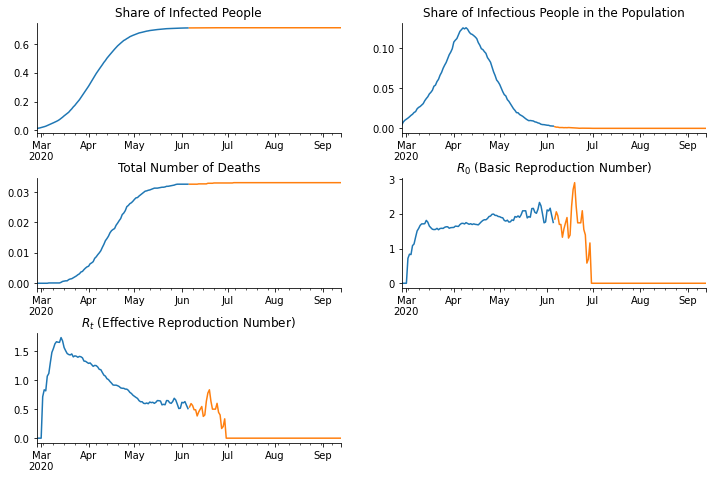
axs[0].set_title("Share of Infected People")
axs[1].set_title("Share of Infectious People in the Population")
axs[2].set_title("Total Number of Deaths")
axs[3].set_title("$R_0$ (Basic Reproduction Number)")
axs[4].set_title("$R_t$ (Effective Reproduction Number)")
axs[5].set_visible(False)
plt.show()