How to simulate

This tutorial helps you to get started with sid by building a simple model. First, it focuses on the core objects which are needed for simulation. Then, the spread of the disease in the artificial population is simulated.

Are we all set? Let’s go!

%matplotlib inline

import warnings

import matplotlib.pyplot as plt
import numpy as np
import pandas as pd

import sid
from sid.config import INDEX_NAMES

warnings.filterwarnings(
    "ignore", message="indexing past lexsort depth may impact performance."
)

The core objects

This section explains the core objects necessary to run a simulation with sid.

The initial_states

Since sid is an agent-based simulator, it needs information on agents or individuals in the model. This information is captured in the initial_states. The initial_states are a pandas.DataFrame where rows represent individuals and columns are characteristics, for example, age, geographic information, etc..

In this context, a state is a single row in the data frame representing an individual at a certain point in time. The characteristics contain all the information needed for the individual to make decisions such as going to work, demanding a test, or for policies to target the individual.

The following states include information on the age of individuals who fall into different age brackets. The age brackets are necessary for some stochastic processes in the model. For example, the probability of staying asymptomatic after an infection is age-dependent since elderly are more likely to experience strong symptoms.

The states also include very broad geographic information of the individuals which only there to speed up simulation.

Note

To give a little bit of background information on the matching algorithm: Later, the tutorial will allow for meetings between two randomly selected people in the model. Instead of searching for a contact partner among all people, it is easier to, first, sample a subset where the partner is in, such as a geographic cluster, and, after that, sample the specific individual.

Once there is an detailed information on the matching algorithm, it will be referenced here. Until then, please consult the API documentation on calculate_infections_by_contacts() and related functions.

We start with 10,000 individuals. Note that all characteristics are converted to categoricals which ensures that values are self-explanatory and save memory.

n_individuals = 10_000
available_ages = [
    "0-9",
    "10-19",
    "20-29",
    "30-39",
    "40-49",
    "50-59",
    "60-69",
    "70-79",
    "80-100",
]

ages = np.random.choice(available_ages, size=n_individuals)
regions = np.random.choice(["North", "East", "South", "West"], size=n_individuals)

initial_states = pd.DataFrame({"age_group": ages, "region": regions}).astype("category")
initial_states.head(5)

	age_group	region
0	10-19	East
1	70-79	West
2	10-19	South
3	10-19	North
4	40-49	East

See also

You can read more about the states in the reference guides.

The contact_models

The contact models are key to how contacts between individuals can be modeled with sid. There are two types of contact models, random and recurrent models:

• Recurrent contact models are used when people belong to a certain group and if they meet this group, they meet all participating members. You would use recurrent models to model school classes, households, and colleagues/work groups.

• Random contact models are used when people do not always meet the same predefined groups, but contacts happen more randomly. Usually, people are more likely to meet a person from their own group, but there is also a lower probability of meeting someone from another group. Groups can be formed by combining any number of characteristics. If we would use age groups, we would say contacts are assortative by age. Each person also has a budget for the number of people she can meet. You would use random contact models, for example, to model meetings during freetime activities, infrequent contacts at work, or acquaintances.

In the following, we define a random contact model which lets each individual in the population meet 0-9 other people each day. The contacts are assortative by age and region since we want to make contacts more likely within the same regions and in the same age groups.

def meet_people(states, params, seed):
    np.random.seed(seed)
    contacts = np.random.choice(np.arange(10), size=len(states))
    return pd.Series(contacts, index=states.index)

contact_models = {
    "meet_people": {
        "model": meet_people,
        "assort_by": ["age_group", "region"],
        "is_recurrent": False,
    }
}

Contact models are stored as a dictionary. Our contact model is called "meet_people" and we define it in another dictionary. The dictionary has the following components.

• "model" holds the function which maps individual characteristics with parameters to a number of contacts which can be an integer or a float – internally the number of contacts is rounded over the whole population while preserving the sum of contacts.

• "assort_by" specifies the variables by which people are more likely to meet each other.

• "is_recurrent" is an indicator for a whether the models represents recurrent or random contacts.

See also

You can read more about contact_models in the references guides.

The params

The parameters are a pandas.DataFrame and include medical and other relevant information. sid offers a prepared database which can be loaded and easily adjusted. The following code can be used for loading.

params = sid.load_epidemiological_parameters()
params.head(5)

			value
category	subcategory	name
health_system	icu_limit_relative	icu_limit_relative	50.00
cd_infectious_true	all	1	0.39
		2	0.35
		3	0.22
		5	0.04

The index is a three dimensional multi index which allows to organize parameters hierarchically. If lower levels are not necessary, it is common to repeat the previous level.

For our model, we need to specify some additional parameters. First, we add the infection probability for our contact model. If a contact happens between an infectious and a susceptible person, the susceptible person becomes infected according to this probability.

params.loc[("infection_prob", "meet_people", "meet_people"), "value"] = 0.05

Similarly, we specify for each contact model how the strength of the assortative matching.

We assume that 90% of contacts are with people from the same region and 50% with contacts from the same age group. It means that the probability of meeting someone from the same age group and region is 0.45. The rest of the probability mass will be split equally between the remaining groups formed by regions and age groups.

params.loc[("assortative_matching", "meet_people", "age_group"), "value"] = 0.5
params.loc[("assortative_matching", "meet_people", "region"), "value"] = 0.9

We further have to specify parameters governing the immunity level and its waning. For a detailed explaination of these parameters see the tutorial notebook on how to model immunity.

immunity_params = pd.read_csv("immunity_params.csv", index_col=INDEX_NAMES)

params = pd.concat((params, immunity_params))

See also

You can read more about params in the references guides.

The initial_conditions

Finally, we need to set the initial_conditions which describes the progression of the disease at the start of the simulation like who is infected or already immune, etc.. sid gives you the ability to start the progression of the infectious disease from patient zero. It also offers a simple interface to come up with complex patterns like individuals in all stages of the disease.

For now, we assume that there are 100 infected individuals and 50 with pre-existing immunity.

initial_conditions = {"initial_infections": 100, "initial_immunity": 50}

See also

More information on the initial_conditions can be found in a dedicated how-to guide.

The simulation

Now, we are going to simulate this population for 200 periods. For that, we define a duration which is a dictionary with a "start" and a "periods" key or a "start" and "end" keys.

duration = {"start": "2020-02-27", "periods": 200}

sid differentiates between the setup of the simulation and the actual simulation. That is why we need to build the simulation() function first.

simulate = sid.get_simulate_func(
    initial_states=initial_states,
    contact_models=contact_models,
    params=params,
    initial_conditions=initial_conditions,
    duration=duration,
    seed=0,
)

After that, the function to simulate the data only depends on the parameters. Now, let us simulate our model!

result = simulate(params=params)

Start the simulation...
2020-09-13: 100%|██████████| 200/200 [00:28<00:00,  7.07it/s]

The result object is a dictionary with two keys:

• "time_series" is a dask.dataframe which holds the data generated by the simulation. Since it is not feasible to hold all the data from the simulation in memory, each day is stored on disk in compressed .parquet files. dask provides a convenient interface to load all files and perform calculation on the data. If you want to work with pandas.DataFrames instead, convert the dask.dataframe to pandas with time_series.compute().

• "last_states" holds a dask.dataframe of the lastly simulated states including all data columns which are usually dropped to save memory. The last_states can be used to resume a simulation.

result.keys()

dict_keys(['time_series', 'last_states'])

Here is a preview for each of the two objects.

result["time_series"].head()

	symptomatic	is_tested_positive_by_rapid_test	infectious	age_group	immunity	newly_vaccinated	cd_infectious_false	newly_infected	ever_infected	date	virus_strain	ever_vaccinated	knows_immune	newly_deceased	region	knows_infectious	needs_icu	new_known_case	n_has_infected	dead
0	False	False	False	10-19	0.0	False	-10001	False	False	2020-02-27	NaN	False	False	False	East	False	False	False	0	False
1	False	False	False	70-79	0.0	False	-10001	False	False	2020-02-27	NaN	False	False	False	West	False	False	False	0	False
2	False	False	False	10-19	0.0	False	-10001	False	False	2020-02-27	NaN	False	False	False	South	False	False	False	0	False
3	False	False	False	10-19	0.0	False	-10001	False	False	2020-02-27	NaN	False	False	False	North	False	False	False	0	False
4	False	False	False	40-49	0.0	False	-10001	False	False	2020-02-27	NaN	False	False	False	East	False	False	False	0	False

result["last_states"].head()

	age_group	region	ever_infected	infectious	symptomatic	needs_icu	dead	pending_test	received_test_result	knows_immune	...	cd_knows_infectious_false_draws	cd_needs_icu_false_draws	cd_needs_icu_true_draws	cd_received_test_result_true_draws	cd_symptoms_false_draws	cd_symptoms_true_draws	group_codes_meet_people	date	period	n_contacts_meet_people
0	10-19	East	True	False	False	False	False	False	False	False	...	-1	-1	-1	2	27	-1	4	2020-09-13	621	5
1	70-79	West	False	False	False	False	False	False	False	False	...	-1	-1	10	4	18	1	31	2020-09-13	621	3
2	10-19	South	False	False	False	False	False	False	False	False	...	-1	15	-1	2	18	-1	6	2020-09-13	621	1
3	10-19	North	False	False	False	False	False	False	False	False	...	-1	-1	-1	1	27	-1	5	2020-09-13	621	0
4	40-49	East	False	False	False	False	False	False	False	False	...	-1	25	-1	1	27	1	16	2020-09-13	621	6

5 rows × 49 columns

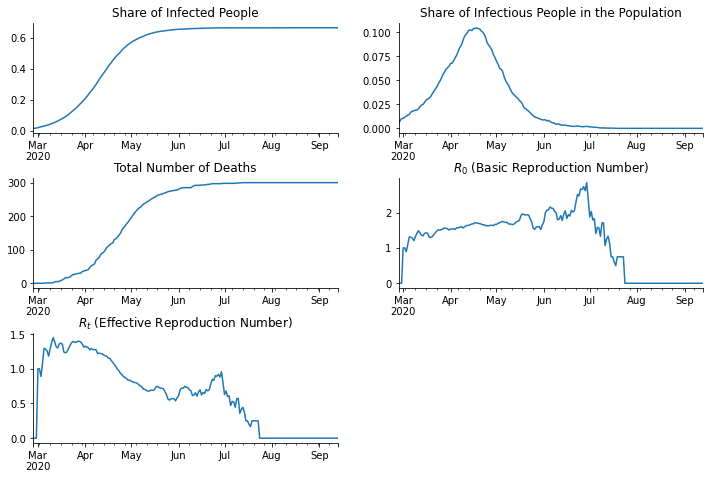
Let us take a look at various statistics of the sample.

df = result["time_series"].compute()

fig, axs = plt.subplots(3, 2, figsize=(12, 8))
fig.subplots_adjust(bottom=0.15, wspace=0.2, hspace=0.4)

axs = axs.flatten()

df.resample("D", on="date")["ever_infected"].mean().plot(ax=axs[0])
df.resample("D", on="date")["infectious"].mean().plot(ax=axs[1])
df.resample("D", on="date")["dead"].sum().plot(ax=axs[2])

r_zero = sid.statistics.calculate_r_zero(df, window_length=7)
r_zero.plot(ax=axs[3])

r_effective = sid.statistics.calculate_r_effective(df, window_length=7)
r_effective.plot(ax=axs[4])

for ax in axs:
    ax.set_xlabel("")
    ax.spines["right"].set_visible(False)
    ax.spines["top"].set_visible(False)

axs[0].set_title("Share of Infected People")
axs[1].set_title("Share of Infectious People in the Population")
axs[2].set_title("Total Number of Deaths")
axs[3].set_title("$R_0$ (Basic Reproduction Number)")
axs[4].set_title("$R_t$ (Effective Reproduction Number)")

axs[5].set_visible(False)

plt.show()